gps-wizard
Alpha Racing
Background
Alpha racing is a merging of GPS technology with the natural back and forth sailing done by most sailboarders around the world. It uses the power of GPS and computing to calculate your best average speed from any point through a gybe and back to the same point.
There are only two rules in Alpha Racing:
- You must get back to a previous position. Because it is not always easy to know exactly where you have been or on what line you sailed into the gybe, a tolerance needs to be applied in the calculations. The term for this tolerance is the Proximity Distance.
- All results must have a total distance covered that is less than or equal to the maximum distance. The software will only calculate results achieved where the total distance covered from start to return is less than or equal to the maximum distance.
Alpha 500 is one of the standard speed categories when speedsurfing, where the proximity distance is 50m and the maximum distance covered is 500m.
No other rules are necessary. As long as you are on a sailboard you can do whatever you like within these two constraints. You can gybe multiple times, you can cross your path multiple times, sail upwind and downwind, you can even tack.
The original website describing alpha racing is no longer online but can be viewed on Wayback Machine.
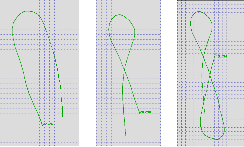
Example Alphas
The image below contains three examples of an alpha 500:
- Typically, alpha 500 runs resemble a U shape so that the finishing speed is maximized after the gybe / turn.
- Crossing the original path is also perfectly acceptable as shown in the second example.
- The third example illustrates two legitimate alphas which actually overlap; i.e. second alpha starts before the first alpha ends.
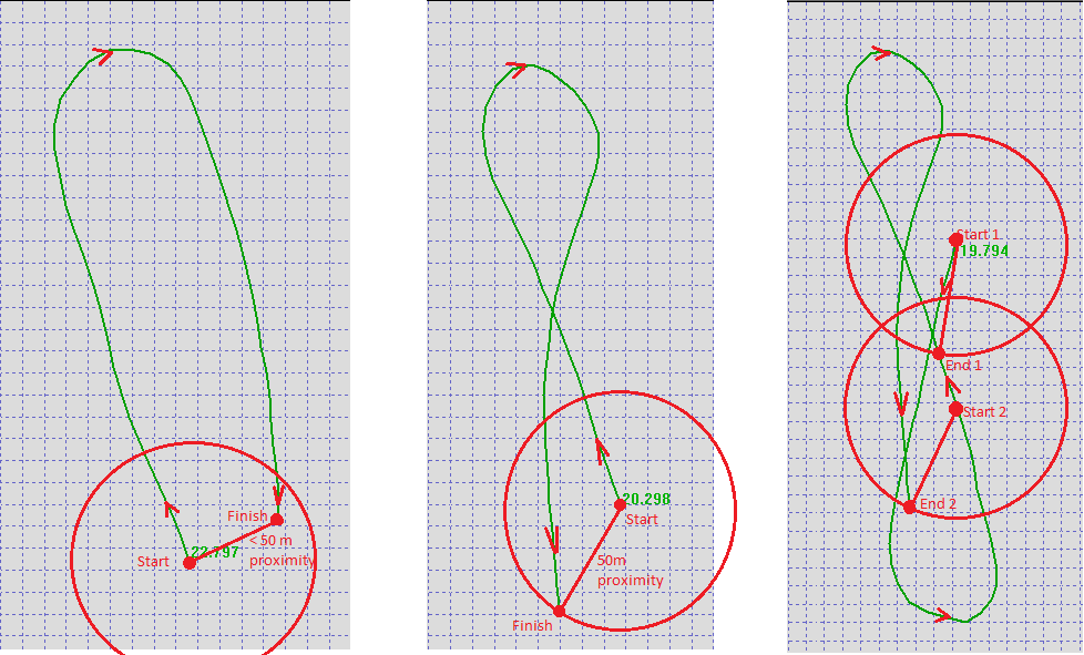
Alpha Detection
There is no prescribed algorithm which dictates how to detect and calculate alpha results within software.
All that matters is that the proximity distance and maximum distance are implemented correctly; 50m and 500m respectively.
The examples from above have been annotated below, showing the significance of the 50m proximity detection.
Implementation
General Principle
The general principle is for every reading from the GNSS receiver, look back over the previous 500m of readings for possible start points of an alpha. Counting backwards over 500m is straightforward (although it is definitely worth using a cache / buffer to facilitate less costly distance calculations) but proximity detection is where things become a little more complicated.
Failure to properly implement the proximity checks can lead to wildly inaccurate alpha results. For example, my APEX Pro reported 27.64 knots on 12 Nov 2021 but it was for a non-qualifying alpha attempt (> 50 m proximity) and the best alpha of the day was actually 21.15 knots.
Using a brute-force approach to determine the possible start points within the required 50m proximity will be computational expensive and there are some major savings to be made through the use of a more intelligent algorithm. Computational costs can be reduced by several orders of magnitude.
Proximity Detection
Proximity detection might appear to be an obvious application for the Haversine formula or Vincenty’s formulae but they are overkill for alpha racing. Whilst either the Haversine formula or Vincenty’s formulae are essential for navigation and when calculating long distances between two points on a globe, they are not required for alpha proximity detection.
This project includes a Python notebook called “haversine_vs_pythagoras” which assesses the accuracy of Pythagorean theorem for the calculation of distances between two points approximately 50m apart, over the entire globe using 1 degree increments in latitude (-90° to + 90°) and longitude (-180° to +180°).
The results of this analysis show that Pythagoras is more than accurate enough at the latitudes which have ever been windsurfed and there is no need to implement the computational expensive Haversine formula or Vincenty’s formulae. Pythagoras produces sub-mm accuracy which is plenty good enough for 50m proximity detection.
One-Time Calculations
A big advantage of using Pythagoras instead of the Haversine formula or Vincenty’s formulae is that the number of relatively costly trig functions (e.g. sin, cos, asin) are reduced during each proximity calculation. These savings add up over time because the search for possible alphas needs to occur after every single reading from the GNSS receiver.
However, this saving in itself is not the biggest advantage. The biggest advantage is that the only remaining trig functions (e.g. calculating the distance from east-west, per degree of longitude at a given latitude, using “cos”) can be cached / buffered and only ever needs to be done once.
This has multiple advantages:
- Total computational cost savings from this optimisation alone will typically be in the order of one to two orders of magnitude.
- The computations are more evenly distributed over time, avoiding particularly high computational spikes towards the end of alphas.
- Time required to analyze alphas in software is greatly reduced and is particularly useful for real-time calculations within a GPS watch.
Minimum Alpha Distance
Although not prescribed in the original definition of alpha racing, software such as GPSResults and the GP3S website (including the COROS auto-sync) implement a “minimum alpha distance”.
A distance of 250m has been chosen by that software as it avoids some minor complexities / grey areas when identifying alpha results and also provides a significant computational saving.
The minimum distance essentially allows the software to skip past the most recent 250m of readings and only consider the prior 250m of data when looking for the start of alpha 500s.
This typically reduces the number of proximity calculations / checks by around 30%.
Angular Differences
Since alphas are essentially a “there and back” (including a gybe / turn) it is useful to look at the angular differences in course over ground (COG) values before calculating the proximity between two points.
A “safe” value to choose for the minimum required angular difference is 90°. This does not affect the alpha results produced but it vastly reduces the number of proximity checks required during a typical speedsurfing session.
In most cases, 120° will suffice but I have identified alpha runs where 115° is required and it is plausible that 90° could potentially be required. The performance benefits from increasing the minimum angular difference further are very small, hence my choice of 90°.
Computational savings (reduced number of proximity checks) can be anywhere between 60% on a small lake and 85% on a large expanse of water.
Overall Savings
The table below shows how the various optimisations affect the number of proximity calculations required during a session.
| 2021-10-20 | 2021-11-12 | 2022-04-04 | |
|---|---|---|---|
| Session summary | Speed session in Portland Harbor; long runs and infrequent turns. | Speed session in Portland Harbor; long runs and infrequent turns. | Foiling session on a small lake; short runs and frequent turns. |
| # Track points | 9,515 | 3,275 | 6,877 |
| # Proximity tests without optimizations | 302,103 | 132,046 | 379,276 |
| # Proximity tests with >= 250m minimum distance | 135,388 | 64,234 | 165,170 |
| # Proximity tests with >= 90° angular difference | 41,647 | 26,045 | 161,046 |
| # Proximity tests with >= 250m and >= 90° angular difference | 28,036 | 18,272 | 115,179 |
The combined savings of the minimum distance (>= 250m) and required angular difference (>= 90°) range from 70% on a small lake to 90% on a large expanse of water. However, these savings are purely related to the number of proximity checks / calculations being performed during the session.
In reality, proximity calculations using pre-cached figures along with Pythagoras will be more than an order of magnitude faster than the regular Haversine formula and Vincenty’s formulae (maybe more) which are computationally expensive and need to be fully evaluated for each pair of potential alpha 500 start and end points.
Overall, the techniques described in this document will lead to computational overheads that are reduced by at least two orders of magnitude, when compared to a brute-force Haversine / Vincenty approaches. The overall processor load will also be spread far more evenly over time and not result in long periods of processor-intensive calculations being performed.
These benefits and savings make the approaches described in this article perfect for real-time calculations within GPS watches such as the models produced by COROS.
All of the sessions below are available on GitHub and were used to test the results of these algorithms. The alpha results are consistent with GPSResults and the number of proximity checks are shown in the table above.
Example Code
Python Implementation
This project contains a Python notebook called “alpha_test” which implements the techniques described throughout this article.
The Python language was chosen for the sake of clarity; it is very readable and the notebook format allows code to be annotated with markdown. Porting this code to other languages should be straightforward and minor tweaks such as the use of a small circular buffer could also be considered for software running in real-time. The pre-calculation of values for Pythagoras is done upfront by the Python but in a GPS watch they would be performed in real-time, once per GNSS reading.
The code that assesses the accuracy of Pythagoras for the purposes of alpha racing is also available in GitHub.
Addendum
Tracks that contains a lot of slow speed may benefit from a slight tweak to the minimum speed logic:
Live 10s > 1 m/s